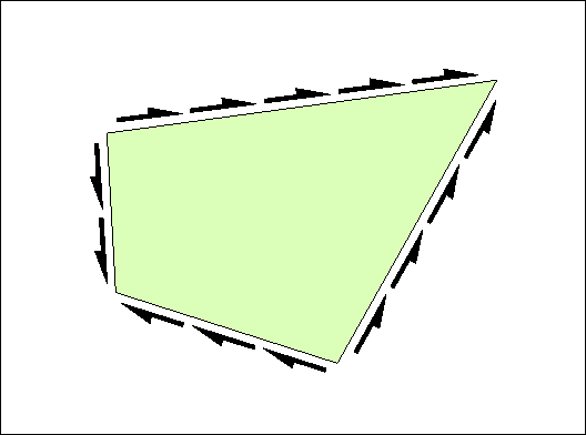
Figure 71: The quadrilateral panels that are used in a linear-elastic analysis have only shear stresses at their edges.
|
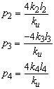
In the linear-elastic formulation of the stringer-panel model only shear stresses occur at the panel edges (see Figure 71). In this way the normal forces are lumped into the stringers where they can be used to dimension the main reinforcement. If the panels for linear analysis would carry part of the normal forces, like the panels for nonlinear simulation do, the reinforcement design would be less efficient. 1 2
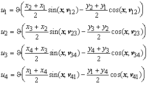
As mentioned before, the discrete element method is adopted to formulate the panel relations. The panel has four edge forces (see Figure 72) and three independent equilibrium relations (in x direction, in y direction and moment equilibrium). So, only one independent parameter b is available to describe the stress field. Each force is accompanied by a displacement so the panel has four degrees of freedom too. Since it has three independent rigid body motions (two translations and one rotation) only one generalised displacement e is left to describe its deformation. The relations are displayed in Figure 73.
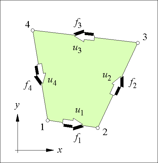 |
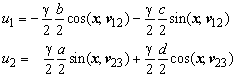
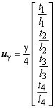
The generalised stress b, which represents the stress field in the panel, is associated with the shear stress t in the middle of the panel. The generalised strain e represents the strain field and is associated with the shear strain g in the middle of the panel. In the subsequent Sections this is defined mathematically.
The relation of the strain g and the stress t is simple since linear-elastic material behaviour is adopted:
t = G g
In this constitutive relation G is the shear modulus of a linear-elastic material.
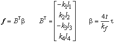
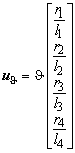
The primary objective of this Appendix is to present the derivation of the stiffness matrix K that relates the vector with panel forces f to the displacement vector u.
f = K u
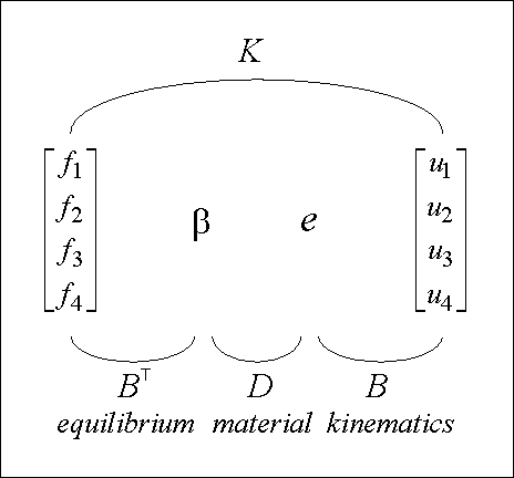 |
As common in the discrete element method the stiffness matrix can be decomposed as
K = BTDB.
In the next Section the equilibrium matrix BT is derived which relates the edge forces f1, f2, f3, f4 with the generalised stress b (see Figure 73). In the third Section the kinematic matrix B is derived which relates the generalised strain e with the edge displacements u1, u2, u3 and u4. In Section 4 the rigidity matrix D is derived. In the last Section the computer code is included for an efficient computation of the panel stiffness matrix.
All derivations are performed in a local two dimensional reference frame. 3 In Appendix 4 the relations are derived for transformation of a panel from a three dimensional space to this two dimensional reference frame.
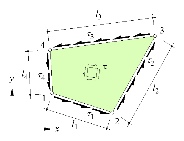
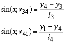
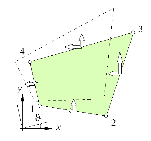
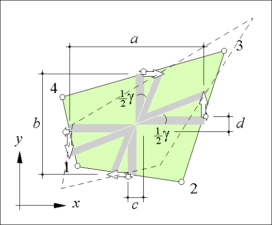
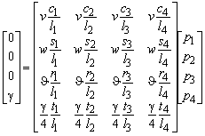
As drawn in Figure 74, the quadrilateral panel is freely positioned in a two dimensional Cartesian reference frame. The panel vertices are numbered 1 to 4 counter-clockwise. At each edge a constant shear traction t1, t2, t3, t4 is present. The positive direction of the edge stresses follows the vertex numbers. This specific layout can be easily implemented in a computer code.
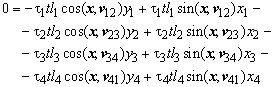
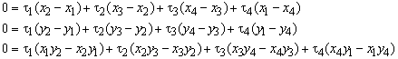
The panel forces have to be in equilibrium in both the x direction and y direction.
![]()
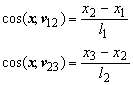
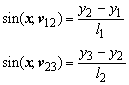
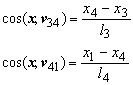
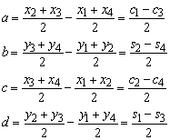
The notation ![]() represents the cosine of the angle of the x axis and the vector from vertex 1 to vertex 2. The panel thickness is denoted t and the lengths of the edges are l1, l2, l3 and l4 as shown in Figure 74.
represents the cosine of the angle of the x axis and the vector from vertex 1 to vertex 2. The panel thickness is denoted t and the lengths of the edges are l1, l2, l3 and l4 as shown in Figure 74.
 |
Moment equilibrium yields the following equation.
Expressing the cosines and sines in the vertex co-ordinates,
we can simplify the equilibrium equations:
The generalised stress b is chosen to be proportional to the average t of the stresses at the panel edges. This average stress can be interpreted as an approximation of the shear stress in the middle of the panel as good as possible in the direction of the edges.
![]()
The four previous equations can be written in matrix notation,
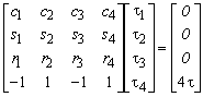
in which the elements are defined according to


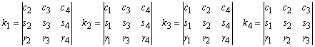
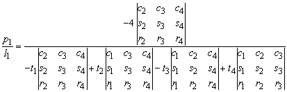
Using Cramers rule t1 can be solved,
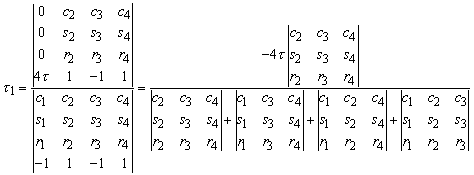
in which the numerator is expanded to the first column and the denominator is expanded to the bottom row. With the notation for the minors
and with![]() this can be conveniently written as
this can be conveniently written as
![]()
Similar expressions can be derived for f2, f3 and f4,
![]()
![]()
![]()
in which
![]()
Defining vector BT and the generalised stress b we can write this as
Thus, the equilibrium relation is derived.
 |
In this Section the kinematic relation between the generalised strain e and the displacements u1, u2, u3 and u4 is derived. The generalised strain of the panel must be a good measure of its shear deformation. As a consequence it should be invariant for rigid body motions.
Three rigid body motions exists, a rigid translation v in the x direction, a rigid translation w in the y direction and a rigid rotation J around the origin.
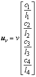
A rigid translation v in the x direction gives the displacement vector uv
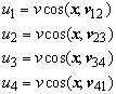
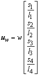
A rigid translation w in the y direction results in the vector uw
![]()
![]()
A rigid rotation J around the origin gives the vector uJ
in which the displacements are linearised (see Figure 75). So, it is only accurate for small rotations which is a valid assumption for concrete structures. In other words geometrically nonlinearities are not included in this panel.
Using the cosines, sines and variables c, s and r defined in the previous Section the rigid motions evaluate to
In Figure 76 the panel is subjected to a homogeneous shear deformation g which results in the edge displacements
![]()
![]()
in which a, b, c and d are dimensions of the panel measured in the panel reference frame (see Figure 76).
Introducing the variables
 |

the displacements can be simplified to
The strain g will be a linear combination of the edge displacements:
![]()
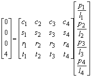
Substituting the four displacement vectors uv, uw, uJ, ug in this relation yields four equations with four unknown coefficients p1, p2, p3, p4.
The first three rows of the matrix correspond with rigid displacements which of course do not give any deformation. Therefore the associated deformation g in the left-hand vector is zero. The last row corresponds with the shear deformation. The relation can be simplified to
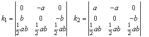
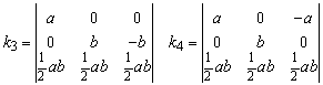
Using Cramers rule p1 can be solved.
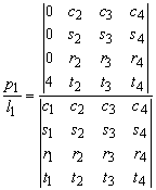
The numerator can be expanded to the first column and the denominator can be expanded to the bottom row.
With the definitions of the minors k1, k2, k3 and k4 from the previous Section this can be simplified to
![]()
Similar expressions can be derived for p2, p3 and p4,
in which
![]()
Recalling the previous definition ![]() and defining the vector B this can be written as
and defining the vector B this can be written as
![]()
Thus, the kinematic relation is derived.
When B of Section 3 is compared to BT derived in Section 2, it appears that they are indeed each others transpose as the notation suggests.
Since
| f = BT b |
b = 4 t t / k | t = G g | g = 4 e / ku | e = B u |
| f = K u | K = BT D B |
obviously the constitutive quantity D is
![]()
The resulting stiffness matrix K is symmetrical and consequently in agreement with the reciprocal theorem of Maxwell. In Section 6 of this Appendix is shown that it can be computed efficiently. Note that extra attention must be given to the computation of kf ku since it has the unit [length10] which can easily produce an overflow of the number memory capacity if small model units are chosen.
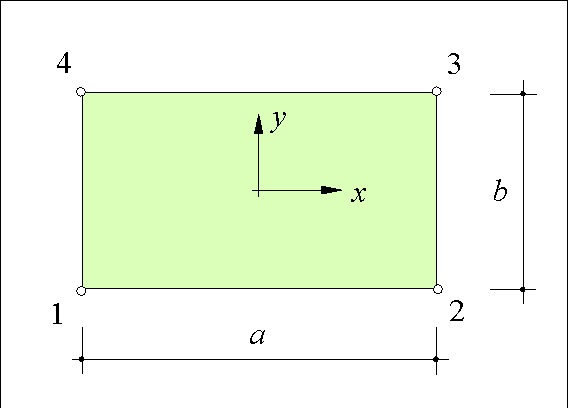
In any practical stringer-panel model, most panels have a rectangular shape. The stiffness matrix of a rectangular shear panel is easily derived and well known [Hoogenboom 1993].

When the vertices of the rectangular panel in Figure 77 are used in the relations of the quadrilateral panel, the minors reduce to
which is evaluated to
 |
![]()
So,

and
![]()
The B vector becomes
![]()
and the resulting stiffness matrix is
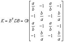
So, when the panel becomes rectangular the relation reduces correctly to the simple relation of a rectangular panel as presented at the start of this Section.
In order to show that the relations can be implemented efficiently, the PASCAL code is added to compute the stiffness matrix of the quadrilateral panel. It consists of only 50 additions or subtractions, 106 multiplications, 2 divisions and 4 square roots. The code uses 47 real number memory locations.
{ --------------- panel stiffness matrix K ------------------- }
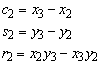
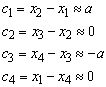
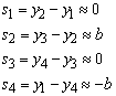
c1:=x2-x1;
c2:=x3-x2;
c3:=x4-x3;
c4:=x1-x4;
s1:=y2-y1;
s2:=y3-y2;
s3:=y4-y3;
s4:=y1-y4;
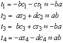
r1:=x1*y2-x2*y1;
r2:=x2*y3-x3*y2;
r3:=x3*y4-x4*y3;
r4:=x4*y1-x1*y4;
l1:=sqrt(c1*c1+s1*s1);
l2:=sqrt(c2*c2+s2*s2);
l3:=sqrt(c3*c3+s3*s3);
l4:=sqrt(c4*c4+s4*s4);
k1:=c2*(s3*r4-s4*r3)-s2*(c3*r4-c4*r3)+r2*(c3*s4-c4*s3);
k2:=c1*(s3*r4-s4*r3)-s1*(c3*r4-c4*r3)+r1*(c3*s4-c4*s3);
k3:=c1*(s2*r4-s4*r2)-s1*(c2*r4-c4*r2)+r1*(c2*s4-c4*s2);
k4:=c1*(s2*r3-s3*r2)-s1*(c2*r3-c3*r2)+r1*(c2*s3-c3*s2);
B[1]:=-k1*l1;
B[2]:= k2*l2;
B[3]:=-k3*l3;
B[4]:= k4*l4;
kf:=k1+k2+k3+k4;
aa:=(c1-c3)*0.5;
bb:=(s2-s4)*0.5;
cc:=(c2-c4)*0.5;
dd:=(s1-s3)*0.5;
ku:=(bb*c1+cc*s1)*k1+(aa*s2+dd*c2)*k2
-(bb*c3+cc*s3)*k3-(aa*s4+dd*c4)*k4;
if (kf<>0.0 and ku<>0.0) then
begin
D:=16.0*G*t/kf/ku;
for i:=1 to 4 do
for j:=1 to 4 do
K[i,j]:=B[i]*D*B[j]
end
else
writeln('Error: Panel is singular. Check panel geometry');
{ --------------- end ---------------------------------------- }
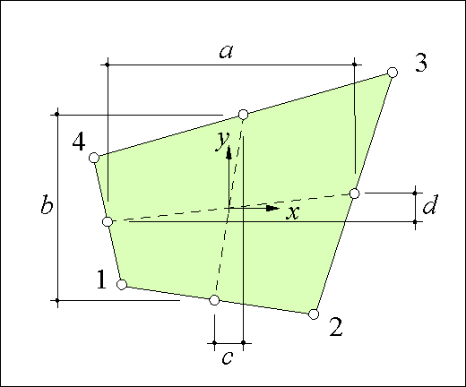
The relations can be approximated if the axis of the panel reference frame are chosen close to the lines through the midsts of opposite edges as Figure 78 shows. In this situation the dimensions c and d are small compared to the other dimensions. They become even smaller if the panel has a more rectangular shape. In that case the dimensions approach to
 |
and
So, the variables t are simplified to
and ku becomes
![]()
This result is theoretically appealing since it introduces extra symmetry of the equilibrium and kinematic relations. It also reduces the computer code with five lines which makes it a few percent faster. However, if these substantial approximations are applied it should be computationally quantified if they can be neglected compared to the approximations that were essential to the derivation. This analysis was not performed and thus the approximations of this Section are not used in the final program.
Perhaps equally a important, is that it would be impossible to display an envelope of panel forces for multiple load combinations if normal forces would occur in the panel.
The theory presented in this Appendix evolved over a number of years. Early literature is [Hoogenboom 1994] and [Lintelo 1995].
A three dimensional treatment is not successful because a panel curved out of plane is only in equilibrium when all panel forces are equal zero.