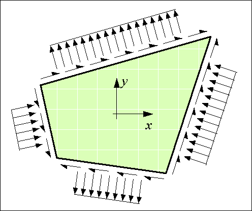
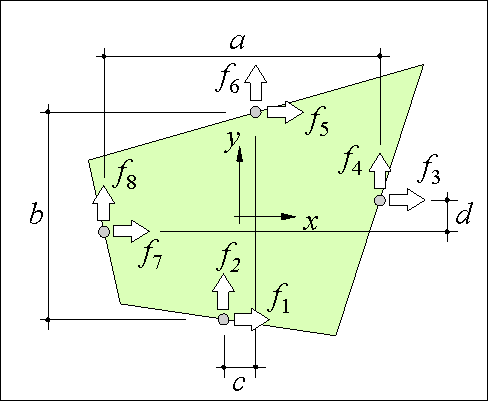
Figure 79: The nonlinear panel has not only shear forces at the edges but normal forces as well.
 |
The panels used in the simulations have not only distributed shear forces acting on the edges but normal forces as well (see Figure 79). Three observations made us decide to include the normal forces and the accompanying displacements in the panel formulation:
First, when panels without normal forces were used to model a box girder beam loaded in pure torsion, we found that the stringers did not get any force. This is in contradiction with experiments in which the longitudinal reinforcement becomes tensioned after cracking of the concrete. The simple reason for the erroneous computation results was that the panels could not dilate since they did not have displacements perpendicular to the edges.
Second, when shear walls were computed with panels without normal forces, a too stiff response was found compared to experiments. This was despite the fact that the stringer strains were used to estimate the normal strains in the panel. We found that also in this case the reason was that the panels could not dilate independently. 1
Finally, the distributed reinforcement contributes to both the shear strength and the normal strength of the material. It would be very conservative to neglect its normal strength since the amount of distributed reinforcement of a wall is often more than the amount of concentrated reinforcement.
Consequently, the panel for simulations has to be able to dilate independently and carry normal stresses as well as shear stresses.
During the simulation process of a stringer-panel model the panel forces are computed for every panel, in every load step and every equilibrium iteration. Consequently, an efficient formulation of the panel behaviour is essential to the speed of the program. In this appendix the panel relations are derived pragmatically using a direct method. 2
The panel must be able to transfer a normal stress at one of the edges to shear stresses at the adjacent edges. So, the stresses in the panel should be at least linear in the x direction for s xx and linear in y for s yy. The following stress field fulfils is used
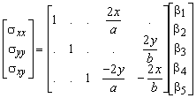
The generalised stresses b1 to b5 each represent a stress mode of the panel as shown in Figure 80. Note that for clarity the zero elements of the matrix are represented by dots. The stress field correctly fulfils the equilibrium requirements

A limitation of the proposed stress field is that it cannot handle a concentrated force in one of the panel vertices. In the stringer-panel model, such a force has to be carried by the stringers and is transferred into the panel with shear stresses.

Figure 80: The panel stress field consists of five independent modes
Starting from this stress field the panel behaviour can be derived with, for example, complementary potential energy as was done for the stringer derivation (see Appendix 1). However, it appeared not possible to obtain a closed form solution because the applied constitutive relation of reinforced concrete cannot be inverted. Consequently, a computational procedure should be used like Newton Raphson, which has shown to be time consuming and not robust. To overcome this problem a different method has been adopted that starts from a displacement field that is consistent with the previously defined stress field.

Figure 81 shows that the panel deformation modes - which are related to the generalised strains e1, e2, e3, e4 and e5 - are in agreement with the previously defined stress modes. The parameters e6, e7 and e8 represent rigid translations and a rigid rotation, respectively.

Figure 81: The panel deformation modes are in agreement with the stress modes.
The objective of this appendix is to present the derivation of a routine with as input the relevant nodal displacements and the panel geometry and as output the panel contribution to the nodal forces and the tangent stiffness matrix. The derivation is carried out in six steps as shown in Figure 82. The steps and variables are described in the subsequent sections.
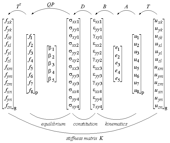
Figure 82: The derivation is organised in six steps from 12 nodal displacements u to 12 nodal forces f.
The panel reference system is derived in Appendix 4. It is uniquely related to the panel geometry and the vertex numbering. Consequently, the panel relations derived in this appendix are independent of the orientation of the panel in space.
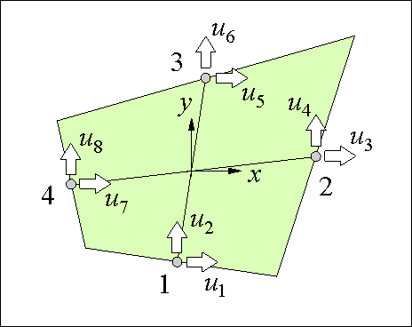
In the first step of the derivation, the twelve global displacements of the nodes with which the panel is connected are rotated to the panel reference system,

where i = 1, 2, 3, 4 is the grip number of the panel and j = j(i) is the number of the connected node in the global model. (see page 15 for more on grips and nodes.) The rotation matrix T is derived in Appendix 4.
As Figure 84 shows the panel dimensions are


For example the variable x1 is the x co-ordinate of vertex 1 in the panel reference system (see Figure 84). As shown in Appendix 4 the same matrix T is used to transform the panel vertices from the global to the local reference system. Of course, the panel dimensions need to be computed only once because they remain constant during a computation.
 |
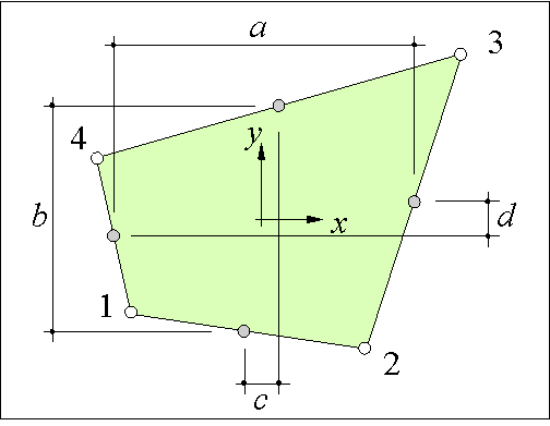 |
| Figure 83: The panel has two displace-ments at each grip, which are computed with a rotation of the nodal displacements to the panel co-ordinate system. The grips are numbered 1 to 4. | Figure 84: The panel vertices are numbered 1 to 4. The vertex co-ordinates are used to define the panel dimensions a, b, c and d. |
In this section, the generalised strains e1 to e5 are derived. They represent the deformation of the panel and are independent of rigid body displacements.
We start with the previously introduced displacement field.

The grip displacements are the displacements of the field at the positions of the grips. The grip co-ordinates are
|
grip 1: grip 2: grip 3: grip 4: |
x = -c/2 x = a/2 x = c/2 x = -a/2 |
y = -b/2 y = d/2 y = b/2 y = -d/2 |
Substitution into the displacement field gives the grip displacements.
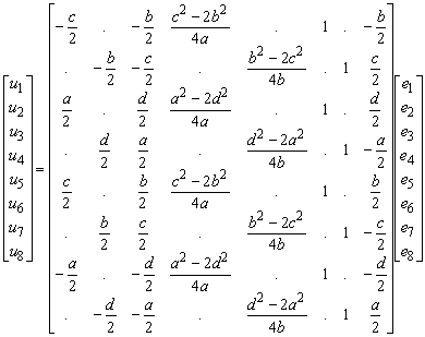
This can be inverted to solve the generalised strains.
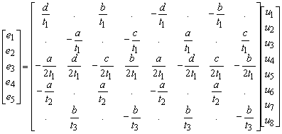
In which
![]()
![]()
![]()
The parameters e6, e7 and e8 are not shown since they represent rigid body displacements which are trivial for the panel deformation. This will be shown in the next section. The latter matrix will be referred to as A.
In the previous section the displacement field is defined and the generalised strains e1 to e5 are expressed in the grip displacements. In this section the strains in the integration points are derived. Before we continue, a few comments have to be made on the number and positions of the integration points.
The most simple approach would be to choose one integration point in the middle of the panel. However, this is not sufficient since the strain tensor for plane stress has three components: Information would be lost if the data of five generalised strains would be transferred to only three strain components. 3 Two integration points would suffice in this respect. However, two points cannot be placed such that any numbering of the panel vertices results in integration points at the same positions. This is important because the panel behaviour should not depend on the vertex numbering. For the same reason, three integration points cannot be used either. Four integration points can be positioned such that any numbering results in integration points at the same positions. So, the panel is designed with four integration points, which contain all together twelve strain components.
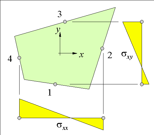
The integration points could be located somewhere in the interior of the panel as is common in the finite element method (Gauß Legendre integration). However, since the strain field is linear in x and y, strains and stresses at the edges become larger than at the integration points. As a consequence, at the edge the stresses can become larger than the ultimate material stress, which is an unsafe approximation with respect to the lower bound theorem of plasticity theory. To be safe the integration points should be chosen at the panel vertices since there the largest strains occur. However, the strain field in the neighbourhood of the vertices is less accurate especially in panels with a highly non rectangular shape. So, as a compromise, the integration points are unconventionally positioned at the midst of the edges as Figure 85 shows.
The co-ordinates of the integration points are coincidentally the same as those of the grips (Newton Côtes integration).
 |
The strain field can be derived from the displacement field with

which are only valid for small strains (geometrical linear relations). As a consequence the panel behaviour is only accurate for small rotations, which is a common and valid assumption for concrete structures. The resulting strain field is
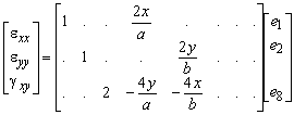
For brevity of the notation not all eight elements e of the right-hand vector are displayed. It is noted that the parameters e6, e7, and e8 indeed represent rigid body displacements since they do not contribute to the strains.
Simulating of the behaviour of experiments showed that the following reduced relation for the shear strains gives more accurate computation results,
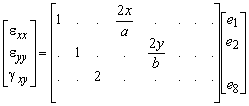
Thus, the shear strain in the panel is constant and equal to the value in its middle. 4
It is not easily explained why this improves the panel behaviour: It was observed in simulations that panels prematurely failed because of large shear stresses at their edges which were not measured in experiments. Instead of attempting to improve the modes 4 and 5 - so that they could capture the observed force flow - we just switched off the disturbing contributions. As a consequence the panel stain field is kinetically not admissible and the shear stresses at the edges are less accurate. In Section 8 of this appendix the latter is taken into account when the grip forces are derived.
Substituting the co-ordinates of the integration points in this result gives the strains in the four integration points.
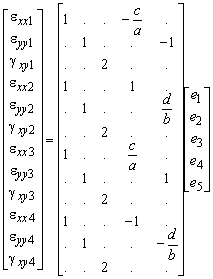
The latter matrix will be referred to as B.
Strains in the integration points are converted to stresses using the modified compression field theory. In this reinforced concrete model, first the principal strains are computed. With the principal strains the principal concrete stresses are computed according to a simple constitutive law. The concrete stresses are transformed to the panel directions and subsequently added to the reinforcement stresses. Finally, the stresses are checked and corrected in order to be in equilibrium in the cracks. Thus, the average concrete stresses sxxc, syyc, sxyc and the average steel stresses sxxs, syys are found in the integration points. The average concrete and steel normal stresses are added to obtain the average material stresses.

Due to the nonlinear material behaviour the panel tangent stiffness matrix will in general not be symmetrical. A further consequence of the material model is that the matrix cannot be derived analytically because the modified compression field theory uses iterations to find equilibrium. Therefore the panel tangent stiffness matrix is computed as explained in Section 10 of this appendix.
In the previous section the stresses in the integration points are derived. In the next section, these stresses are used to derive the grip forces. In this section the twelve stress components in the four integration points are reduced to a stress field described by five generalised stresses b1 to b5. Only five independent generalised stresses are available since the eight grip forces are related with three equilibrium equations. As explained in Section 2 the panel stress field is
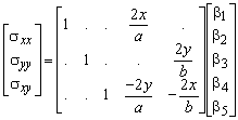
In the middle of the panel is x = y = 0, which results in the stresses

The co-ordinates of the integration points are substituted into the stress field which relates the stresses at the integration points to the generalised stresses.
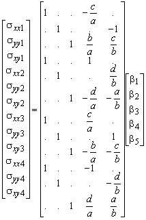
This can be written as
s = L b
The vector with generalised stresses b needs to be solved but we cannot invert L since the system has more equations than unknown. The method of least squares was adopted to derive a best fit of the stress field to the integration point stresses.
b = (LT L) -1LT s
The evaluated equations are too large to be included here. For the special panel geometry in which c = d = 0 it simplifies to

So, the stresses in the middle of the panel are the averages of the stresses in the integration points.

The stress tensor can be displayed in the principal directions with

|

|
In this, s1 is the largest principal stress, s2 is the smallest principal stress and a is the angle between the x axis and the direction of the largest principal stress.
At first glance it may seem that in this Section information is lost due to the reduction from twelve to five variables. However, the opposite is true since the equilibrium relations are introduced, which improve the stress field calculated from the strains. Nevertheless, the derived stress field is not used in the remainder of the text as explained in the next section.
|
|
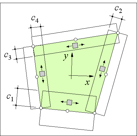
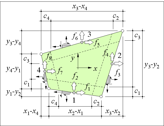
| Figure 86: Since the material of stringers and panels overlap, it must be avoided that part of the stresses appears both in the panel and in its adjacent stringers. | Figure 87: The stresses at the panel edges are in equilibrium with the grip forces. |
In the previous Section the stress field and the generalised stresses were derived. From the generalised stresses, the grip forces can be found with for example virtual work. A complication is that parts of the stresses in the material of the panel are already assigned to the stringers: As Figure 86 shows, the stress in the direction of a stringer contributes to the virtual work of the stringer and cannot be assigned to the panel too.
In this Section a more straight forward method is employed to derive the grip forces directly from the stresses in the integration points. Since the stress field is linear in any direction the resulting force per unit of thickness at the edge can be simply found by multiplying the stress in the integration point with the projected length of the edge. This is in fact a one point Gauß integration of a stress component along the edge.
For example, the horizontal grip force f3 is computed from the stresses in integration point 2 (see Figure 87). The grip force consists of three contributions: The horizontal reinforcement stress sxx2s multiplied with the vertical edge length y3 - y2. The horizontal concrete stress sxx2c multiplied with a reduced horizontal edge length (y3 - y2) - c1- c3 and the horizontal concrete shear stress sxy2c multiplied with the horizontal edge length x3 - x2.

![]()
![]()
![]()
![]()

The tildes (~) at some of the grip forces f will be explained further on. The relations are only exact for a rectangular panel. When the panel is not rectangular - as in Figure 87 - the relations are a sufficiently accurate approximation of the influence of the stringer widths c.
The grip forces that are found above are generally not in equilibrium for three reasons. 5 First, the grip forces are based on the stresses in the integration points and not on the generalised stresses. Second, a linear stress field at an edge produces not only a grip force but a moment as well. These moments at the edges are not yet taken into account. Third, part of the edge stresses have been cut because they were assigned to the stringers.
It is decided to correct the forces f1, f4, f5 and f8 related mainly to shear at the panel edges. These forces are labelled with a tilde (~) showing that they are not yet in equilibrium. The correction is minimised using the method of least squares. Therefore an object function is introduced
![]()
subject to the restrictions of the equilibrium equations. Force equilibrium in the x, y direction and moment equilibrium around the origin yields (see Figure 88)

The restrictions can be added to the function using Lagrange multipliers.

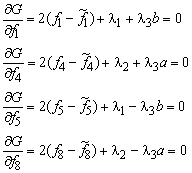
The function G is minimised with respect to the forces and the Lagrange multipliers.
![]()
![]()
![]()
From these equations the forces in equilibrium can be solved.
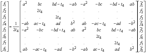
In this t4 = a2 + b2. The latter matrix will be referred to as Q. Thus, any set of panel forces ![]() is transformed to equilibrium.
is transformed to equilibrium.
 |
![]()
As a check, the forces can be again transformed to equilibrium, which should give the same result:
![]()
So,
![]()
which property the matrix indeed appears to possess.
Finally, the grip forces are rotated from the panel co-ordinate system to the global co-ordinate system

in which i = 1, 2, 3, 4 is the grip number and j = j(i) the related node number. The nodal forces are either added to the global force vector or used for the computation of the panel tangent stiffness matrix.
The previously derived panel relation can be easily implemented in a computer program. The routine computes the panel forces directly from the panel displacements. It consists of 156 multiplications, 21 divisions, and 174 additions and subtractions.
{ --------------- panel dimensions --------------------------- }
a:=(x2+x3-x1-x4)*0.5;
b:=(y3+y4-y1-y2)*0.5;
c:=(x3+x4-x1-x2)*0.5;
d:=(y2+y3-y1-y4)*0.5;

{ --------------- panel grip displacements u ----------------- }
for i:=1 to 4 do
begin
  k:=2*i;
  l:=3*i;
  u[k-1]:=t11*ug[l-2]+t12*ug[l-1]+t13*ug[l];
  u[k]  :=t21*ug[l-2]+t22*ug[l-1]+t23*ug[l];
end

{ --------------- generalised strains e ---------------------- }
t1:=a*b-c*d;
t2:=a*a-c*c;
t3:=b*b-d*d;
t4:=t2*0.5+t3;
t5:=t3*0.5+t2;
if (t1=0.0 or t4=0.0 or t5=0.0) then
  writeln(‘Error: Panel dimensions are singular.’);
e1:=( d*u[1]+b*u[3]-d*u[5]-b*u[7])/t1;
e2:=(-a*u[2]-c*u[4]+a*u[6]+c*u[8])/t1;
e3:=(-a*u[1]+d*u[2]-c*u[3]+b*u[4]+
      a*u[5]-d*u[6]+c*u[7]-b*u[8])*0.5/t1;
e4:=(-u[1]+u[3]-u[5]+u[7])*a/t4;
e5:=( u[2]-u[4]+u[6]-u[8])*b/t5;

{ --------------- strains in integration points -------------- }
if a=0.0 or b=0.0 then
  writeln(‘Error: Panel has no dimensions. Check panel shape.’);
exx[1]:=e1-c/a*e4;
eyy[1]:=e2-e5;
gxy[1]:= 2.0*(e3+b/a*e4+c/b*e5);
exx[2]:=e1+e4;
eyy[2]:=e2+d/b*e5;
gxy[2]:=2.0*(e3-d/a*e4-a/b*e5);
exx[3]:=e1+c/a*e4;
eyy[3]:=e2+e5;
gxy[3]:=2.0*(e3-b/a*e4-c/b*e5);
exx[4]:=e1-e4;
eyy[4]:=e2-d/b*e5;
gxy[4]:=2.0*(e3+d/a*e4+a/b*e5);

{ --------------- stresses in integration points ------------- }
for i:=1 to 4 do
begin
  mcft(PanNr, exx[i], eyy[i], gxy[i];
       var sxxc[i], syyc[i], sxy[i], sxxs[i], syys[i]: real);
  sxx[i]:=sxxc[i]+sxxs[i];
  syy[i]:=syyc[i]+syys[i]
end;

{ --------------- generalised stresses b --------------------- }
b1:=(sxx[1]+sxx[2]+sxx[3]+sxx[4])*0.25;
b2:=(syy[1]+syy[2]+syy[3]+syy[4])*0.25;
b3:=(sxy[1]+sxy[2]+sxy[3]+sxy[4])*0.25;

{ --------------- panel grip forces f ------------------------ }
t1:=y2-y1; t2:=x2-x1; t3:=t2-c2-c4;
if t3<0.0 then t3:=0.0;
f[1]:=(sxx[1]*t1-sxy[1]*t2)*t;
f[2]:=(-syyc[1]*t3-syys[1]*t2+sxy[1]*t1)*t;
t1:=y3-y2; t2:=x3-x2; t3:=t1-c3-c1;
if t3<0.0 then t3:=0.0;
f[3]:=(sxxc[2]*t3+sxxs[2]*t1-sxy[2]*t2)*t;
f[4]:=(-syy[2]*t2+sxy[2]*t1)*t;
t1:=y3-y4; t2:=x3-x4; t3:=t2-c2-c4;
if t3<0.0 then t3:=0.0;
f[5]:=(-sxx[3]*t1+sxy[3]*t2)*t;
f[6]:=(syyc[3]*t3+syys[3]*t2-sxy[3]*t1)*t;
t1:=y4-y1; t2:=x4-x1; t3:=t1-c1-c3;
if t3<0.0 then t3:=0.0;
f[7]:=(-sxxc[4]*t3-sxxs[4]*t1+sxy[4]*t2)*t;
f[8]:=(syy[4]*t2-sxy[4]*t1)*t;

t0:=2.0*(a*a+b*b);
t1:=(a*(f[1]-f[5])-b*(f[4]-f[8]))/t0;
t2:=(c*(f[2]-f[6])+d*(f[3]-f[7]))/t0;
t3:=(f[3]+f[7])/2.0;
t4:=(f[2]+f[6])/2.0;
f[1]:= a*t1+b*t2-t3;
f[4]:=-b*t1+a*t2-t4;
f[5]:=-a*t1-b*t2-t3;
f[8]:= b*t1-a*t2-t4;

{ --------------- global nodal forces fg --------------------- }
for i=1 to 4 do
begin
  k:=2*i;
  t1:=f[k-1];
  t2:=f[k];
  l:=3*i;
  fg[l-2]:=t1*t11+t2*t21;
  fg[l-1]:=t1*t12+t2*t22;
  fg[l  ]:=t1*t13+t2*t23;
end
{ --------------- end ---------------------------------------- }
The elements of the tangent stiffness matrix K are defined as
![]()
K can be evaluated analytically with
K = Q P D B A
The matrix Q is defined on page 145 and the matrix P represents the relations on page 142 and 143. Together Q and P embody the equilibrium of the panel. The matrices A and B are derived in Section 3 and 4, respectively. They embody the kinematic relations of the panel. The constitutive matrix D represents the material behaviour. It is only explicitly available when the material is approximated linear-elastic.
As explained before, the tangent stiffness matrix of the panel is not derived analytically but computed by the program. This is necessary because the constitutive model contains iterations. It is also convenient because in this way the computer code can be easily adapted which has shown to be very important.
The algorithm for computing the tangent matrix is printed below.
{ --------------- degrees of freedom numbers ----------------- }
for i:=1 to 4 do
begin
  k:=3*Pan[PanNr].NodeNr[i];
  l:=3*i;
  v[l-2]:=k-2;
  v[l-1]:=k-1;
  v[l  ]:=k;
end

{ --------------- grip forces -------------------------------- }
for i:=1 to 12 do
  u[i]:=ug[v[i]];

PanelForces(PanNr, u, f);

{ --------------- panel tangent stiffness matrix ------------ }
for i:=1 to 12 do
begin
  u[i]:=u[i]+d;
  PanelForces(PanNr, u, fd);
  for j:=1 to 12 do
  begin
    K[j,i]:=(fd[j]-f[j])/d;
    u[i]:=u[i]-d
  end
end
{ --------------- end ---------------------------------------- }
A comparable stiffness matrix formulation according to the finite element theory would consist of four multiplications of two 8 times 3 matrices and a 3 times 3 and matrix. Moreover, it is has to be transformed to the global reference system which requires two multiplications with a 8 times 12 matrix. Excluding the assembly of the matrices this involves 2976 multiplications and 2384 additions.
As mentioned before the routine PanelForces of the previous section consists of 156 multiplications, 21 divisions, and 174 additions and subtractions. To compute the stiffness matrix and the panel forces it is called 13 times. Together this involves 2301 multiplications or divisions and 2262 additions or subtractions. So, the derived panel is somewhat faster than a standard finite element.
 |
Of course, the panel formulation is an approximation of the exact mechanical behaviour of a reinforced concrete panel. The ultimate check of the formulation is the comparison with experiments as described in Chapter 3. The formulation can also be checked directly using the following four properties that are inherent to the exact behaviour:
In this section it is shown that the derived panel formulation fulfils property 1 and 2 for small deformations and rotations. Property 3 is not fulfilled which will be illustrated below. Finally, it is shown that the formulation correctly complies with property 4.
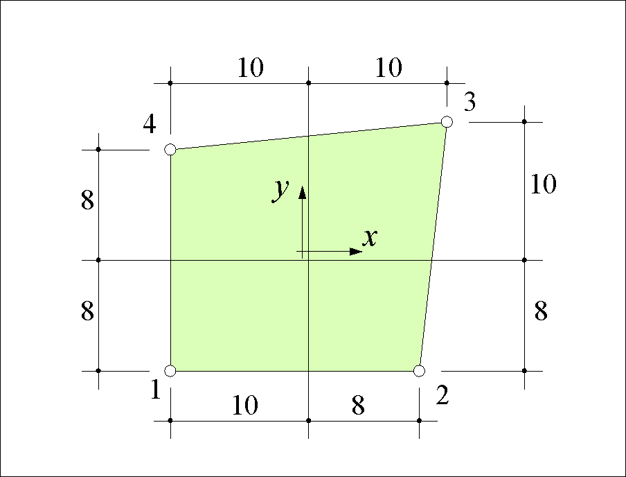
We start with a specific panel geometry and stringer margins so that the calculated matrices can be displayed.


![]()
The panel dimensions become


The equilibrium matrix QP evaluates to

The kinematic matrix BA evaluates to
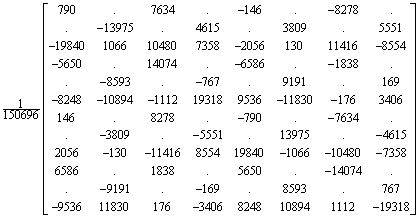
The matrices fulfil the kinematic and the equilibrium requirements as shown next (property 1 and 2, respectively).
The kinematic condition is that no strains may occur for rigid body displacements. Rigid body displacements are a translation v in the x direction
u1 = u3 = u5 = u7 = v
or a translation w in the y direction
u2 = u4 = u6 = u8 = w
or a rotation J around the middle of the panel

The latter are the linearised displacements due to a rigid panel rotation. So, they are only accurate for small rotations.
The rigid body displacements can be written as
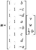
The latter matrix will be called CT. For this example C evaluates to

If the kinematic matrix BA is multiplied with CT a 12 times 3 matrix appears with only zero elements.
BA CT = 0
This shows that the panel strains, stresses and grip forces correctly equal zero when the panel undergoes rigid body displacements.
The equilibrium conditions have already been formulated on page 144:


Again the matrix C appears. When C is multiplied with QP a 3 times 12 matrix appears with only zero elements.
C QP = 0
This shows that the grip forces are correctly in equilibrium.
Subsequently, the reciprocity of the panel formulation is discussed. Reciprocity is defined as the property of linear structures that a load at one position can be interchanged with the resulting displacement at another position. 6 It can be easily shown that this property is equivalent to symmetry of the stiffness matrix K.
K = QP D BA
In general the panel tangent stiffness matrix K is not symmetric for two reasons: First, the matrix D is not symmetric due to the nonlinear material behaviour. Second, the kinematic matrix QP does not equal the transpose of the equilibrium matrix BA. 7
![]()
So, the panel does not fulfil property 3 mentioned above. 8 This is clearly illustrated with the calculated panel stiffness matrix assuming linear material behaviour and a Poisson’s ratio v = 0:
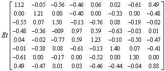
For this example of a panel slightly deviating from a rectangular shape, the approximation of the symmetry is acceptable.
Finally, we show that the formulation correctly reduces to the relations for a rectangular panel with linear material behaviour (property 4).
In the case of only shear stiffness the material matrix D is extremely sparse.
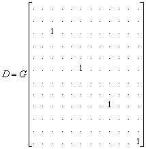
In this, G is the shear modulus. The dimensions of a rectangular panel are


The resulting panel stiffness matrix is
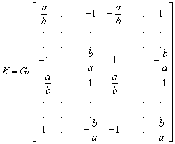
which is consistent with the result of a panel with only shear stiffness as derived in Appendix 2.
For a panel with only normal stiffness the material matrix becomes
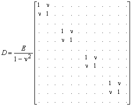
If the stringer margins are c1 = c2 = c3 = c4 = 0 the stiffness matrix evaluates to
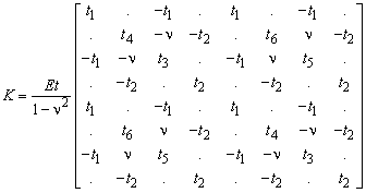
in which


The resulting matrix is symmetric and it produces grip forces that are in equilibrium and invariant for rigid displacements. For all displacement modes it can be manually checked that the matrix produces correct grip forces.
In finite element literature this phenomena is referred to as locking.
In a collective effort we have tried many formulations of the panel. Derivations were based on the virtual labour equation, on complementary potential energy, on the Hellinger Reissner functional, with shape functions for displacement or stress fields on curvilinear co-ordinates or in curvilinear directions. The formulation of this appendix is considered to be the best because it is simple in method and result, which makes it fast and less vulnerable for errors. Detailed studies of the panel formulation can be found in [Lintelo 1995], [Heeres January 1996] and [Heeres June 1996].
If this is implemented the panel would be able to deform in some modes without using energy. This is frequently referred to as hourglass modes.
In finite element literature a similar adaptation of the strain field became known as selective integrations because the same effect is obtained when the shear stresses are evaluated in only one integration point in the middle of the element.
The underlying reason is that the displacement field with which we started the derivation is in general not exact. In theory we could adapt the displacement field such that equilibrium is met. Indeed in finite element literature, elements have been derived with internal nodes for which the displacements are determined with equilibrium iterations. This is necessary for simple elements which otherwise show pathological locking.
In the stringer formulation equilibrium iterations were used too (see Appendix 1). Because it took considerable effort before these iterations were robust, we decided to adopt another approach: The panel grip forces are adapted such that they are in equilibrium.
For example, Load a cantilever beam at its tip and measure at the same time its displacement at some other point of the beam. Subsequently, put the load where the displacement was measured and the tip will get the displacement measured before.
It is noted that equality of the transposed is a sufficient but not necessary condition for symmetry. It was observed that the stiffness matrix sometimes becomes symmetric despite the fact that QP <> (BA)T. For example the rectangular panels at the end of Section 12 are symmetric.
Instead of the relation K = QP D BA we could have used the standard finite element theory which yields K = ĽOt (BA)T D BA. In this t is the panel thickness and O the panel surface area (In the example of this section O = 322). This formulation gives a symmetric matrix, however, the finite element formulation does not include the panel margins, it shows an annoying locking and it does not reduce correctly for a rectangular panel.